Exploratory data analysis¶

Last updated: 2020-12-22

Background¶

Flanker Data We’ll be working with data from a similar flanker experiment as we used in Assignment 2. However, in Assignment 2 we gave you a “sanitized” version of the data, where we had done a bit of clean-up to extract just the information we wanted you to work with. In this assignment you’ll get experience starting with the raw data and extracting the necessary information yourself.

–PSYO 3505 Fall 2019 Assignment 2 cell1

Read file and check it¶

import pandas as pd
import numpy as np
import matplotlib.pyplot as plt

First of all we need input and examine the data

subjects = ['001_2015_05_22_11_30',
            '002_2015_05_25_14_36',
            '003_2015_05_28_14_09'
           ]

in_file = subjects[0]+'/'+subjects[0]+'_data.txt'

#input to data_frame
df = pd.read_csv(in_file)

df.head(5)

	id\tyear\tmonth\tday\thour\tminute\tgender\tage\thandedness\twait\tblock\ttrial\ttarget_location\ttarget\tflankers\trt\tresponse\terror\tpre_target_response\tITI_response\ttarget_on_error
0	001\t2015\t05\t22\t11\t30\tm\t25\tr\t3.24\tpra...
1	001\t2015\t05\t22\t11\t30\tm\t25\tr\t3.24\tpra...
2	001\t2015\t05\t22\t11\t30\tm\t25\tr\t3.24\tpra...
3	001\t2015\t05\t22\t11\t30\tm\t25\tr\t3.24\tpra...
4	001\t2015\t05\t22\t11\t30\tm\t25\tr\t3.24\tpra...

looks like not very well, we need add escape character. Typically, I prefer read csv file directly and then check the head.

df = pd.read_csv(in_file,sep = '\t')
df

	id	year	month	day	hour	minute	gender	age	handedness	wait	...	trial	target_location	target	flankers	rt	response	error	pre_target_response	ITI_response	target_on_error
0	1	2015	5	22	11	30	m	25	r	3.240	...	1	left	black	incongruent	NaN	NaN	NaN	False	False	0.023
1	1	2015	5	22	11	30	m	25	r	3.240	...	2	right	black	incongruent	0.550	black	True	False	False	0.023
2	1	2015	5	22	11	30	m	25	r	3.240	...	3	up	white	incongruent	0.565	white	True	False	False	0.024
3	1	2015	5	22	11	30	m	25	r	3.240	...	4	up	black	congruent	0.453	black	True	False	False	0.024
4	1	2015	5	22	11	30	m	25	r	3.240	...	5	down	black	congruent	0.442	black	True	False	False	0.023
...	...	...	...	...	...	...	...	...	...	...	...	...	...	...	...	...	...	...	...	...	...
187	1	2015	5	22	11	30	m	25	r	1.627	...	28	left	white	congruent	0.349	white	True	False	False	0.024
188	1	2015	5	22	11	30	m	25	r	1.627	...	29	right	white	congruent	0.371	white	True	False	False	0.023
189	1	2015	5	22	11	30	m	25	r	1.627	...	30	up	black	incongruent	0.549	black	True	False	False	0.023
190	1	2015	5	22	11	30	m	25	r	1.627	...	31	left	white	neutral	0.463	white	True	False	False	0.023
191	1	2015	5	22	11	30	m	25	r	1.627	...	32	right	black	neutral	0.430	black	True	False	False	0.023

192 rows × 21 columns

look at the head and tail again

df.head(5)

	id	year	month	day	hour	minute	gender	age	handedness	wait	...	trial	target_location	target	flankers	rt	response	error	pre_target_response	ITI_response	target_on_error
0	1	2015	5	22	11	30	m	25	r	3.24	...	1	left	black	incongruent	NaN	NaN	NaN	False	False	0.023
1	1	2015	5	22	11	30	m	25	r	3.24	...	2	right	black	incongruent	0.550	black	True	False	False	0.023
2	1	2015	5	22	11	30	m	25	r	3.24	...	3	up	white	incongruent	0.565	white	True	False	False	0.024
3	1	2015	5	22	11	30	m	25	r	3.24	...	4	up	black	congruent	0.453	black	True	False	False	0.024
4	1	2015	5	22	11	30	m	25	r	3.24	...	5	down	black	congruent	0.442	black	True	False	False	0.023

5 rows × 21 columns

df.tail(5)

	id	year	month	day	hour	minute	gender	age	handedness	wait	...	trial	target_location	target	flankers	rt	response	error	pre_target_response	ITI_response	target_on_error
187	1	2015	5	22	11	30	m	25	r	1.627	...	28	left	white	congruent	0.349	white	True	False	False	0.024
188	1	2015	5	22	11	30	m	25	r	1.627	...	29	right	white	congruent	0.371	white	True	False	False	0.023
189	1	2015	5	22	11	30	m	25	r	1.627	...	30	up	black	incongruent	0.549	black	True	False	False	0.023
190	1	2015	5	22	11	30	m	25	r	1.627	...	31	left	white	neutral	0.463	white	True	False	False	0.023
191	1	2015	5	22	11	30	m	25	r	1.627	...	32	right	black	neutral	0.430	black	True	False	False	0.023

5 rows × 21 columns

Then we check have missing value

print(pd.isna(df).sum())

id                     0
year                   0
month                  0
day                    0
hour                   0
minute                 0
gender                 0
age                    0
handedness             0
wait                   0
block                  0
trial                  0
target_location        0
target                 0
flankers               0
rt                     2
response               2
error                  2
pre_target_response    0
ITI_response           0
target_on_error        0
dtype: int64

Data cleaning¶

Obviously, we need to remove missing data by appling

.dropna() method

df = df.dropna()
print(pd.isna(df).sum())

id                     0
year                   0
month                  0
day                    0
hour                   0
minute                 0
gender                 0
age                    0
handedness             0
wait                   0
block                  0
trial                  0
target_location        0
target                 0
flankers               0
rt                     0
response               0
error                  0
pre_target_response    0
ITI_response           0
target_on_error        0
dtype: int64

This experiment has ‘practice’, the main idea is giving participants a chance to figure out the experiment. But we do not need it in our EDA. Not all experiments have ‘practice’ .

value = df[‘block’] print(value.unique())

df = df[df.block!='practice']
value = df['block']
print(value.unique())

['1' '2' '3' '4' '5']

Then we found ‘rt’ column is not milliseconds and need to convert

df['rt']

   0.528
   0.419
   0.514
   0.406
   0.502
       ...  
  0.349
  0.371
  0.549
  0.463
  0.430
Name: rt, Length: 160, dtype: float64

df['rt'] = df['rt']*1000
print(df['rt'])

   528.0
   419.0
   514.0
   406.0
   502.0
       ...  
  349.0
  371.0
  549.0
  463.0
  430.0
Name: rt, Length: 160, dtype: float64

‘rt’ is our interested variable, but In most behavioural studies, RTs are not normally distributed, so we need to Examining the RT distribution

df['rt'].describe()

count    160.00000
mean     465.16875
std      101.47170
min      314.00000
25%      392.25000
50%      454.00000
75%      505.25000
max      845.00000
Name: rt, dtype: float64

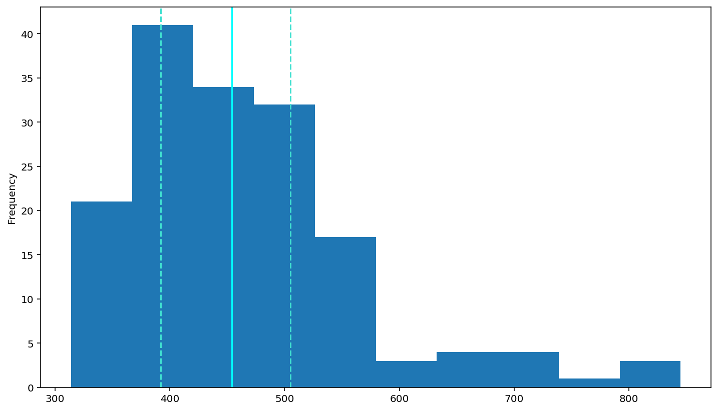
plot a histogram of RTs

df['rt'].plot(kind='hist')

# add a solid line at the median and dashed lines at the 25th and 75th percentiles (done for you)
plt.axvline(df['rt'].describe()['25%'], 0, 1, color='turquoise', linestyle='--')
plt.axvline(df['rt'].median(), 0, 1, color='cyan', linestyle='-')
plt.axvline(df['rt'].describe()['75%'], 0, 1, color='turquoise', linestyle='--')

# Rememebr to use plt.show() to see your plots (often they show anyway, but with some garbagy text at the top)
plt.show()

Analyzing relationships between variables¶

According to above figure, the histogram look not follow normal distribution, Looks like right skewed. Because the data sets have low ‘high value
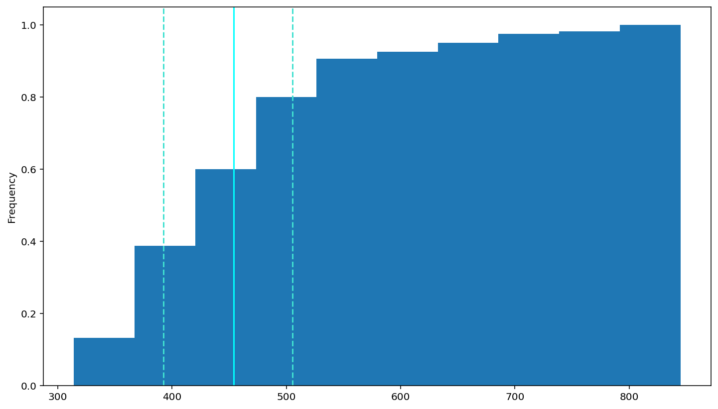
check the cdf

df['rt'].plot(kind = 'hist',cumulative = True, density =True)
# add a dashed oragne line at the median
plt.axvline(df['rt'].describe()['25%'], 0, 1, color='turquoise', linestyle='--')
plt.axvline(df['rt'].median(), 0, 1, color='cyan', linestyle='-')
plt.axvline(df['rt'].describe()['75%'], 0, 1, color='turquoise', linestyle='--')

plt.show()

How should we do in this situation. The course tells me :

While the skew in the RT data makes sense, for the reasons described above, it’s problematic when running statistics on the data. This is because many conventional statistical tests, like t-tests and ANOVAs, assume that the data are normally distributed. Using skewed data can cause unreliable results.

For this reason, many researchers apply some transformation to RTs to make their distribution more normal (statistically normal, that is). A common one is to take the logarithm of the RT values: log(RT)log(RT); another is to take the inverse: 1/RT.

—PSYO 3505 Fall 2019 Assignment 2 cell40

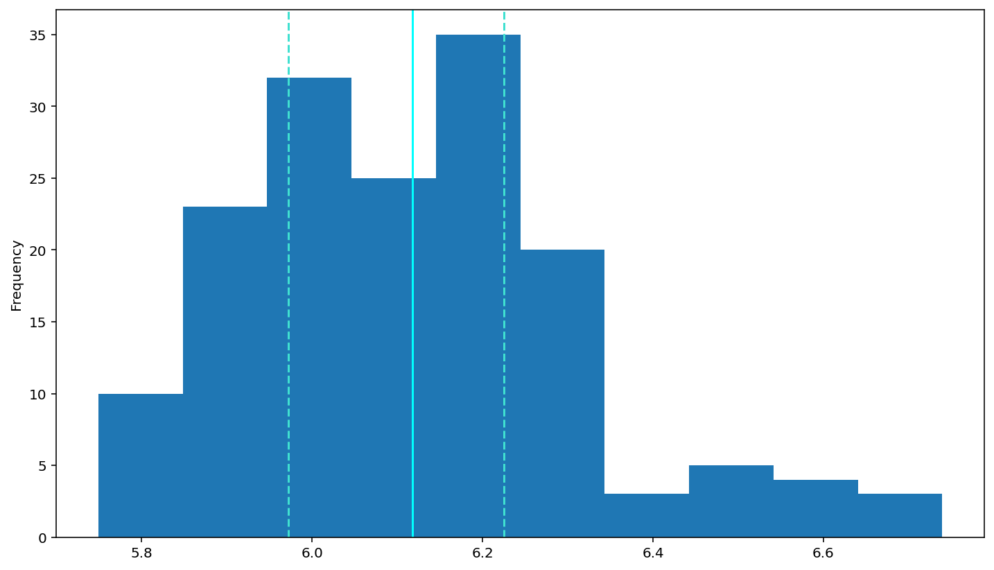
So, for log(RT)

# log-transform the rt data (done for you) 
df['logrt'] = np.log(df['rt'])

# put your plotting code here
# YOUR CODE HERE
df['logrt'].plot(kind='hist')

# add a solid line at the median and dashed lines at the 25th and 75th percentiles (done for you)
plt.axvline(df['logrt'].describe()['25%'], 0, 1, color='turquoise', linestyle='--')
plt.axvline(df['logrt'].median(), 0, 1, color='cyan', linestyle='-')
plt.axvline(df['logrt'].describe()['75%'], 0, 1, color='turquoise', linestyle='--')

# Rememebr to use plt.show() to see your plots (often they show anyway, but with some garbagy text at the top)
plt.show()

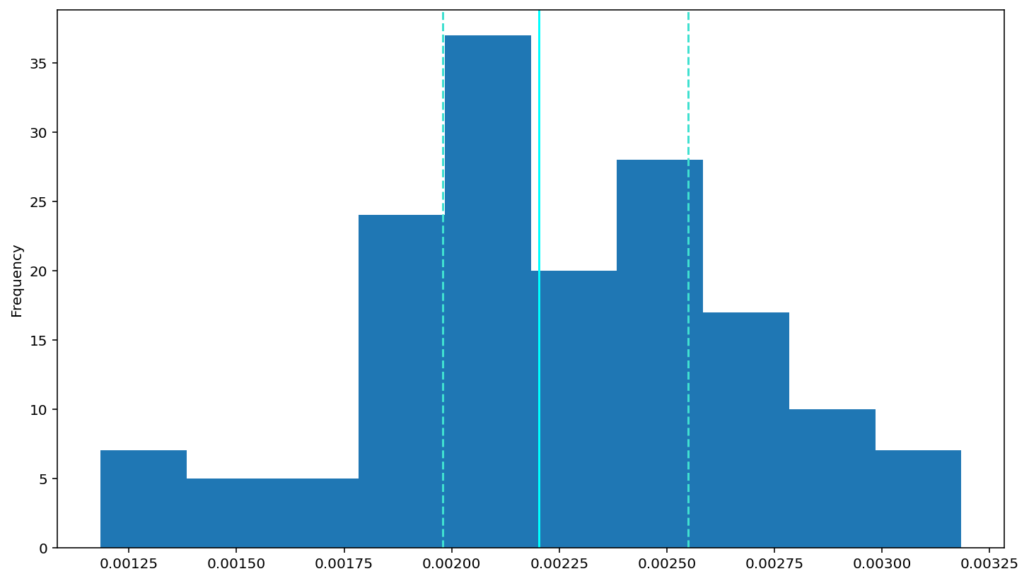
inverse: \(1/RT\)

df['invrt'] = 1/(df['rt'])

df['invrt'].plot(kind='hist')
# add a solid line at the median and dashed lines at the 25th and 75th percentiles (done for you)
plt.axvline(df['invrt'].describe()['25%'], 0, 1, color='turquoise', linestyle='--')
plt.axvline(df['invrt'].median(), 0, 1, color='cyan', linestyle='-')
plt.axvline(df['invrt'].describe()['75%'], 0, 1, color='turquoise', linestyle='--')

# Rememebr to use plt.show() to see your plots (often they show anyway, but with some garbagy text at the top)
plt.show()

After that, we want to explore the data will be on errors and reaction times (RTs).

Recall that these data are from a “flanker” experiment in which participants had to respond with a left or right button press, depending on whether the target (centre) arrow pointed left or right. The target arrow was flanked with two arrows on either side that were either congruent (pointed in same direction) or incongruent (opposite direction).

—PSYO 3505 Fall 2019 Assignment 2 cell48

Tip

You can found more information about flanker experiment in this article ‘Flanker and Simon effects interact at the response selection stage’

rt_mean = df.groupby(by = 'flankers')[['rt','error']].agg('mean')
rt_mean = rt_mean.drop('neutral')
rt_mean

	rt
flankers
congruent	452.60
incongruent	466.05

Generate a table for accuracy (the error column).

correct = df.groupby(by = 'flankers')[['error']].agg('sum')
correct.columns = ['Correct']
correct = correct.drop('neutral')
correct

	Correct
flankers
congruent	40
incongruent	34

showing the accuracy rate

total= df.groupby(by = 'flankers')[['error']].agg('count')
correct = df.groupby(by = 'flankers')[['error']].agg('sum')
number = correct[:2]/total[:2]
number.columns = ['Accuracy']
number

	Accuracy
flankers
congruent	1.00
incongruent	0.85

Visualization¶

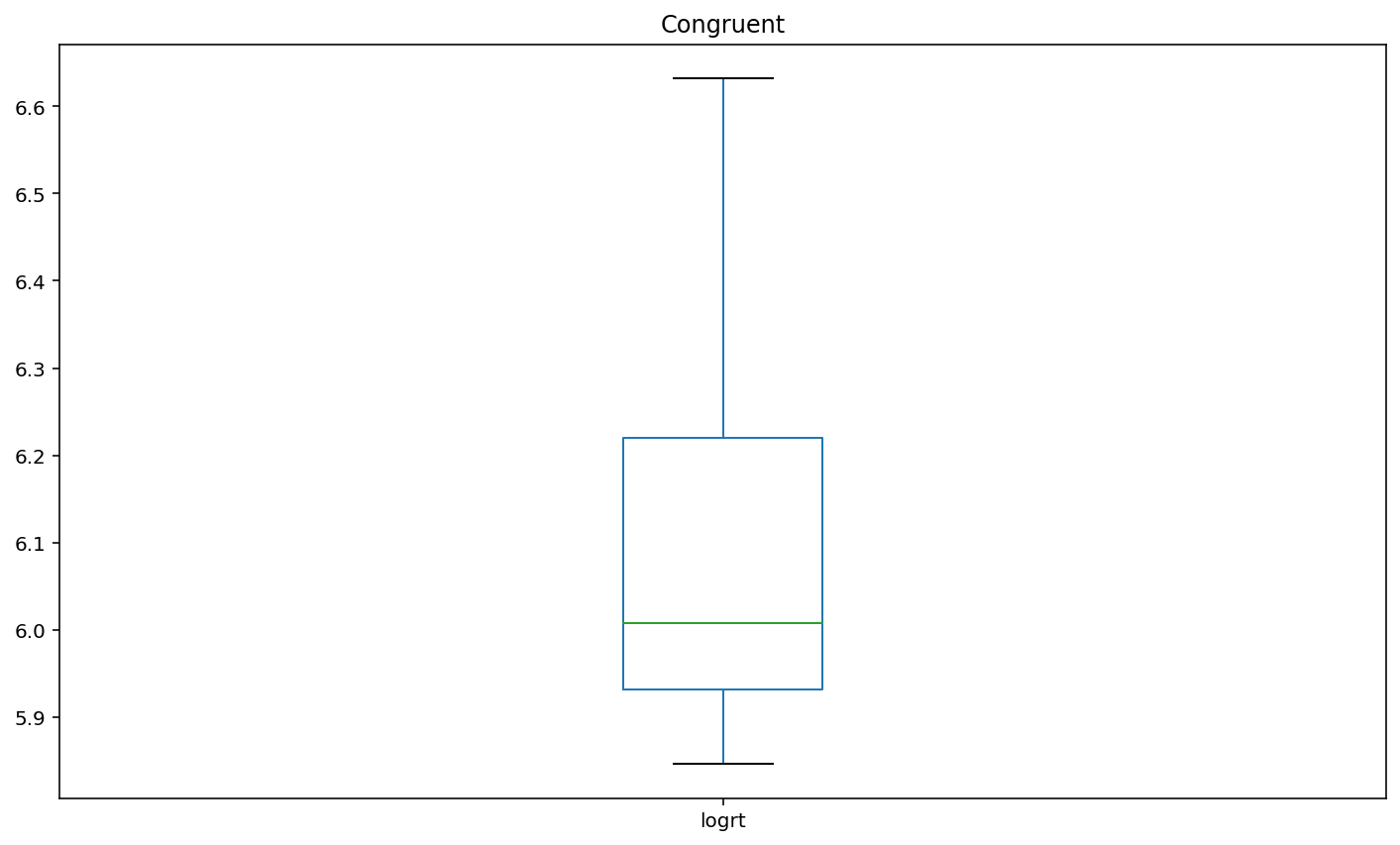
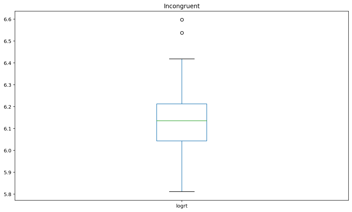
Plot box plots of the log-transformed RT data (logrt) for each flanker conditio

boxplot1 = df.loc[df['flankers']=='congruent','logrt'].plot(kind = 'box',title = 'Congruent')
plt.show()
boxplot2 = df.loc[df['flankers']=='incongruent','logrt'].plot(kind = 'box',title = 'Incongruent')
plt.show()

Interpretation¶

Basis of EDA, I can say incongruent flankers would lead to slower and less accurate responses. according to the participant results, the congruent condition has 100% accuracy and 452.60 (mean) response time. Incongruent condition has 85% accuracy and 466.05 (mean) response time.

So far, we end EDA methods (basic).

Through this assignment, I learned the basic steps of data analysis. Especially,EDA methods:
Read files
Data cleaning
Analyzing relationships between variables
Visualization
Interpretation

References¶

[1] NESC 3505 Neural Data Science, at Dalhousie University. Textbook
[2] NESC 3505 Neural Data Science, at Dalhousie University. Assignment 3
[3] An Extensive Step by Step Guide to Exploratory Data Analysis

This Demo and the attached files from course PSYO/NESC 3505 Neural Data Science, at Dalhousie University. You should not disseminate, distribute or copy.
I am NOT post inappropriate or copyrighted content, advertise or promote outside products or organizations
© Copyright 2020.PSYO/NESC 3505 FAll 2020 https://dalpsychneuro.github.io/NESC_3505_textbook/intro.html
For demonstration purposes only

Art of Thinking